Building an Unsupervised Machine Learning Trading Algorithm with Python

Introduction
Downloading and Preparing Data
Feature Engineering and Technical Indicators
Calculating Returns and Factor Exposure
Clustering for Asset Selection
Portfolio Construction with Efficient Frontier Optimization
Performance Visualization
Conclusion

Introduction

With the increasing complexity of financial markets, unsupervised learning techniques like clustering offer a powerful approach to asset selection and portfolio optimization. In this article, we develop a systematic trading strategy using Python, leveraging clustering methods to categorize assets based on their characteristics and then optimizing our portfolio using the efficient frontier. This strategy aims to outperform the market by dynamically selecting assets from different clusters and adjusting allocations based on risk-return metrics.

Downloading and Preparing Data

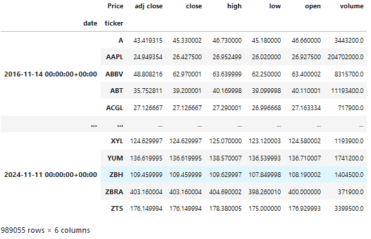
To begin, we need data on S&P 500 stock prices, covering at least several years to ensure sufficient historical context. Using Yahoo Finance, we download daily price data for each stock in the S&P 500 index, which forms the basis for our analysis and feature engineering.

from statsmodels.regression.rolling import RollingOLS
import pandas_datareader.data as web
import matplotlib.pyplot as plt
import statsmodels.api as sm
import pandas as pd
import numpy as np
import datetime as dt
import yfinance as yf
import pandas_ta
import warnings
warnings.filterwarnings('ignore')

sp500 = pd.read_html('https://en.wikipedia.org/wiki/List_of_S%26P_500_companies')[0]

sp500['Symbol'] = sp500['Symbol'].str.replace('.', '-')

symbols_list = sp500['Symbol'].unique().tolist()

end_date = '2024-11-12'

start_date = pd.to_datetime(end_date)-pd.DateOffset(365*8)

df = yf.download(tickers=symbols_list,
                 start=start_date,
                 end=end_date).stack()

df.index.names = ['date', 'ticker']

df.columns = df.columns.str.lower()

df

This code snippet demonstrates how to download stock data using the yfinance library and prepare it for further analysis.

After loading the data, we calculate various technical indicators for each stock. These indicators capture different market dynamics and provide essential features for the clustering model.

Feature Engineering and Technical Indicators

In this section, we compute technical indicators that highlight key market characteristics, including volatility, relative strength, and trend. The indicators chosen here are Garman-Klass volatility, RSI, Bollinger Bands, ATR, and MACD, all of which help quantify asset behavior.

Calculating Technical Indicators

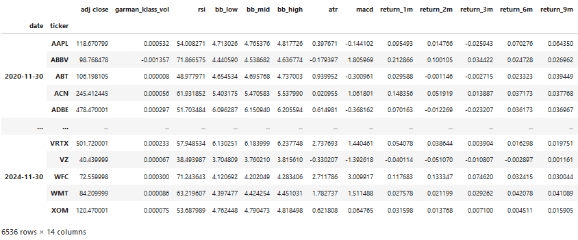
Following the data preparation step, we calculate the Garman-Klass volatility, RSI, Bollinger Bands, ATR, MACD, and dollar volume for each stock in the dataset. These indicators provide valuable insights into price action and market dynamics, enabling us to categorize stocks effectively through clustering.

df['garman_klass_vol'] = ((np.log(df['high'])-np.log(df['low']))**2)/2-(2*np.log(2)-1)*((np.log(df['adj close'])-np.log(df['open']))**2)

df['rsi'] = df.groupby(level=1)['adj close'].transform(lambda x: pandas_ta.rsi(close=x, length=20))

df['bb_low'] = df.groupby(level=1)['adj close'].transform(lambda x: pandas_ta.bbands(close=np.log1p(x), length=20).iloc[:,0])
                                                          
df['bb_mid'] = df.groupby(level=1)['adj close'].transform(lambda x: pandas_ta.bbands(close=np.log1p(x), length=20).iloc[:,1])
                                                          
df['bb_high'] = df.groupby(level=1)['adj close'].transform(lambda x: pandas_ta.bbands(close=np.log1p(x), length=20).iloc[:,2])

def compute_atr(stock_data):
    atr = pandas_ta.atr(high=stock_data['high'],
                        low=stock_data['low'],
                        close=stock_data['close'],
                        length=14)
    return atr.sub(atr.mean()).div(atr.std())

df['atr'] = df.groupby(level=1, group_keys=False).apply(compute_atr)

def compute_macd(close):
    macd = pandas_ta.macd(close=close, length=20).iloc[:,0]
    return macd.sub(macd.mean()).div(macd.std())

df['macd'] = df.groupby(level=1, group_keys=False)['adj close'].apply(compute_macd)

df['dollar_volume'] = (df['adj close']*df['volume'])/1e6

df

Each indicator provides a unique perspective on price action, enabling us to categorize stocks effectively through clustering.

Calculating Returns and Factor Exposure

Returns calculation is essential for assessing performance over multiple time horizons. Here, we calculate monthly returns over different periods, creating features that reflect price momentum and mean reversion trends.

def calculate_returns(df):

    outlier_cutoff = 0.005

    lags = [1, 2, 3, 6, 9, 12]

    for lag in lags:

        df[f'return_{lag}m'] = (df['adj close']
                              .pct_change(lag)
                              .pipe(lambda x: x.clip(lower=x.quantile(outlier_cutoff),
                                                     upper=x.quantile(1-outlier_cutoff)))
                              .add(1)
                              .pow(1/lag)
                              .sub(1))
    return df
    
    
data = data.groupby(level=1, group_keys=False).apply(calculate_returns).dropna()

#make date timee zone naive
data.index = data.index.set_levels([data.index.levels[0].tz_localize(None), data.index.levels[1]])

data

The code snippet above demonstrates how to calculate returns over different time horizons and handle outliers to ensure robust performance metrics.

These returns are crucial for understanding asset performance and identifying factors that drive returns over time.

Machine Mearning Clustering for Asset Selection

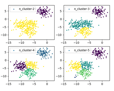
Using unsupervised K-Means clustering, we group stocks with similar behaviors and characteristics. Clustering allows us to categorize assets, ultimately enabling more informed portfolio decisions by selecting assets from different groups to enhance diversification and capture varied market movements.

Implementing K-Means Clustering

Clusterin is a powerful technique for identifying patterns in data and grouping similar assets together. By applying K-Means clustering to our dataset, we can categorize stocks based on their features and characteristics.

from sklearn.cluster import KMeans

from sklearn.cluster import KMeans

# Drop `cluster` column if it exists
data = data.drop('cluster', axis=1, errors='ignore')

def get_clusters(df):
    # Perform clustering without specifying initial centroids
    df['cluster'] = KMeans(n_clusters=4, random_state=0).fit(df).labels_
    return df

# Apply clustering to each date group
data = data.dropna().groupby('date', group_keys=False).apply(get_clusters)

data

The code snippet above demonstrates how to implement K-Means clustering on our dataset, grouping stocks into distinct clusters based on their features and characteristics.

Portfolio Construction with Efficient Frontier Optimization

To maximize returns while controlling for risk, we construct a portfolio based on efficient frontier optimization. We use PyPortfolioOpt to select an optimal asset allocation that achieves the highest Sharpe ratio.

We will create a function that optimizes portfolio weights using the PyPortfolioOpt package and the EfficientFrontier optimizer to maximize the Sharpe ratio. To optimize the weights of a given portfolio, we need to provide the last year's prices to the function. We will also apply a single stock weight bounds constraint for diversification, setting the minimum weight to half of an equal weight and the maximum weight to 10% of the portfolio.

Optimizing Asset Weights

Below is the Python function that optimizes the weights of a given portfolio using the EfficientFrontier optimizer from the PyPortfolioOpt package. The function takes the historical prices of the assets as input and returns the optimized weights for the portfolio.

from pypfopt.efficient_frontier import EfficientFrontier
from pypfopt import risk_models
from pypfopt import expected_returns

def optimize_weights(prices, lower_bound=0):
    
    returns = expected_returns.mean_historical_return(prices=prices,
                                                      frequency=252)
    
    cov = risk_models.sample_cov(prices=prices,
                                 frequency=252)
    
    ef = EfficientFrontier(expected_returns=returns,
                           cov_matrix=cov,
                           weight_bounds=(lower_bound, .1),
                           solver='SCS')
    
    weights = ef.max_sharpe()
    
    return ef.clean_weights()

The function optimize_weights calculates the expected returns and covariance matrix of the assets based on historical prices and optimizes the portfolio weights to maximize the Sharpe ratio. The weight_bounds parameter sets the lower and upper bounds for the asset weights, ensuring diversification and risk control.

Performance Visualization

Finally, we plot the cumulative returns of our strategy over time, comparing it to the benchmark (S&P 500). This visualization provides insights into the strategy's performance and its ability to generate alpha over the benchmark.

import matplotlib.ticker as mtick
import numpy as np
import matplotlib.pyplot as plt

plt.style.use('ggplot')

# Ensure portfolio_df contains only numeric values (filter out non-numeric columns if any)
portfolio_df = portfolio_df.apply(pd.to_numeric, errors='coerce').fillna(0)  # Convert non-numeric data to NaN and fill with 0

# Calculate cumulative returns for each column in the DataFrame
portfolio_cumulative_return = np.exp(np.log1p(portfolio_df).cumsum()) - 1

# Plot cumulative returns up to a specific date
portfolio_cumulative_return[:'2024-10-29'].plot(figsize=(16, 6))

plt.title('Unsupervised Learning Trading Strategy Returns Over Time')
plt.gca().yaxis.set_major_formatter(mtick.PercentFormatter(1))  # Format y-axis as percentage
plt.ylabel('Return')
plt.show()

The code snippet above demonstrates how to visualize the cumulative returns of our trading strategy over time, providing insights into its performance relative to the benchmark.

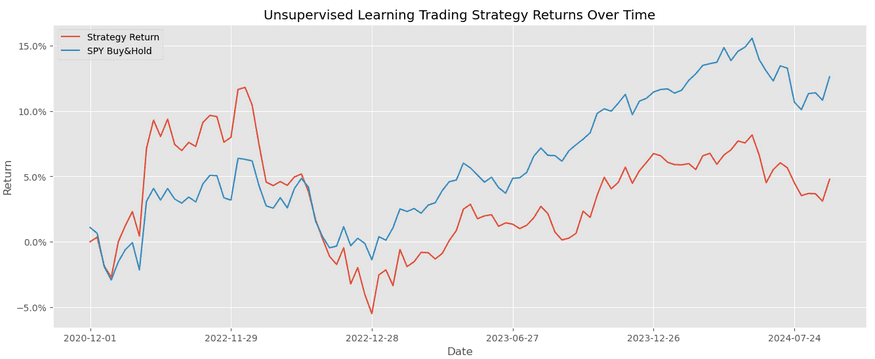
The graph represents a performance comparison between an unsupervised learning-based trading strategy (using K-Means clustering) and a traditional "buy-and-hold" strategy for the S&P 500 index (represented by SPY). Here's a breakdown of the key observations:

Strategy Return vs. SPY Buy-and-Hold:

The red line represents the cumulative return of the K-Means clustering strategy over time, while the blue line represents the SPY Buy-and-Hold strategy.
The K-Means clustering strategy starts with lower returns and experiences more variability over time compared to the buy-and-hold strategy.

Performance Patterns:

Early Period (Late 2020 to Mid-2021): Both strategies initially perform similarly, with some minor fluctuations. However, the K-Means strategy shows an early drop in cumulative returns while SPY maintains steady growth.
Mid-2021 to Early 2023: The buy-and-hold strategy for SPY steadily climbs, reflecting a generally upward trend in the market. Meanwhile, the K-Means clustering strategy experiences more variability, including a notable increase in early 2022 before facing a decline in late 2022.
Late 2023 to Mid-2024: Both strategies diverge more clearly in performance. The SPY Buy-and-Hold strategy exhibits a strong upward trend, reaching about 15% cumulative return by mid-2024, while the clustering strategy shows more fluctuations, ending around 5%.

Volatility:

The K-Means clustering strategy is generally more volatile, experiencing more frequent and sharper ups and downs compared to the SPY Buy-and-Hold strategy. This suggests that while clustering may help capture short-term trends or momentum, it is more sensitive to market changes.

Overall Performance:

By mid-2024, the SPY Buy-and-Hold strategy outperforms the K-Means clustering strategy with a cumulative return of about 15% versus 5% for the clustering strategy. This could imply that while K-Means clustering can help capture certain patterns in the data, it might not be as effective in maintaining consistent growth over a longer period compared to a straightforward buy-and-hold approach.

Potential Insights:

The K-Means strategy’s performance could reflect the clustering model’s sensitivity to changing market conditions. If the model is not retrained or adjusted for market shifts, it may fail to capture long-term trends effectively.
Additionally, the K-Means clustering may be effective for short-term trading or in volatile markets where pattern recognition is beneficial, but it may struggle in stable upward-trending markets.

Conclusion

By implementing an unsupervised learning-based trading strategy, we have explored how clustering and portfolio optimization can lead to efficient and systematic asset allocation. This approach demonstrates the value of machine learning in quantitative finance and highlights the potential for advanced analytics to drive trading decisions.

This analysis shows that the K-Means clustering approach might be able to capture short-term market fluctuations, but over the longer term, a buy-and-hold strategy on a major index like SPY tends to provide more stable and higher cumulative returns. Further refinement of the clustering strategy, possibly by incorporating other indicators or updating clusters more frequently, could help improve performance.

Next Steps

Model Refinement: Experiment with different clustering algorithms, feature sets, or optimization techniques to enhance the strategy's performance.
Risk Management: Implement risk controls, stop-loss mechanisms, or position sizing strategies to manage downside risk and improve overall portfolio stability.
Backtesting: Conduct extensive backtesting to validate the strategy's performance under various market conditions and refine the model based on historical data.
Real-Time Implementation: Develop a pipeline for real-time data ingestion, model updates, and trade execution to deploy the strategy in live trading environments.